Lift Testing with Interrupted Time Series: A Marketing Case Study#

Running Lift Tests When You Have No Control Group#

In marketing analytics, lift tests (also known as incrementality tests) are experiments designed to measure the true causal impact of advertising campaigns. These results are crucial for:

Validating marketing attribution models
Calibrating Media Mix Models (MMM) to improve accuracy
Making informed budget allocation decisions

The gold standard for lift testing is a randomized controlled trial with treatment and control groups. However, this is not always possible. When running national-level campaigns (such as TV advertising in the UK), there may be no geographic control group available since the entire market receives the treatment simultaneously.

This notebook demonstrates how to use Interrupted Time Series (ITS) analysis to conduct a lift test and generate the statistical outputs needed for downstream applications like MMM calibration. ITS is particularly valuable when:

You’re running national campaigns with no geographic controls
You need to measure the incremental impact of a campaign above baseline activity
You want to feed experimental results into your MMM to improve parameter estimates

Connection to Media Mix Modeling

The lift test results from this notebook (mean lift and standard deviation) can be directly integrated into MMM frameworks like PyMC-Marketing to calibrate saturation curves and improve attribution accuracy. See the PyMC-Marketing lift test calibration documentation for details on how to use these results.

The Business Scenario#

Imagine you are managing marketing for a national brand in the UK. Your marketing mix includes:

Baseline TV Brand Awareness: Continuous, low-level TV spend to maintain brand presence
TV Promo Campaign: A 4-week high-spend campaign for a new product launch or seasonal promotion
Digital Paid Advertising: Ongoing digital marketing efforts
Radio: Steady radio advertising

The TV promo campaign represents a significant investment - both in producing a new advertisement and in media buying to air it during prime time. The spend during this promotional period is much higher than your baseline TV spend.

The Challenge: Because the TV campaign runs nationally, you don’t have a clean control group. You can’t compare sales in “treated” vs “untreated” regions.

The Solution: Use Interrupted Time Series analysis to fit sales before the campaign. We can then use that model to estimate the counterfactual estimate of what the sales would have been without the campaign. Comparing that and the actual sales gives us an estimate of the causal impact of the promo campaign.

Lift Test Outputs#

A successful lift test provides statistical estimates of campaign effectiveness that can be used for both immediate decision-making and model calibration. Using ITS analysis, we’ll generate:

Primary Lift Test Results (for MMM Calibration)#

Absolute Lift with Uncertainty: The total incremental units (sales, conversions, etc.) attributable to the campaign, expressed as a posterior distribution with mean and standard deviation. This is the key output needed for MMM calibration.

Additional Business Metrics#

Percentage Lift: The percentage increase in the outcome variable compared to the counterfactual baseline
Return on Investment (ROI): The financial return from the campaign relative to spend

All metrics include full uncertainty quantification through Bayesian inference, providing not just point estimates but complete probability distributions. This uncertainty information is essential for:

MMM Calibration: Informing how strongly the lift test should constrain model parameters
Decision Making: Understanding the range of plausible campaign effects
Risk Assessment: Quantifying confidence in positive/negative ROI

Structure of This Notebook

This notebook is organized into the following sections:

Setup and Imports: Load required packages
Part I: Data Simulation: Generate synthetic marketing data with realistic patterns
- Define time periods and intervention dates
- Create media spend data for multiple channels
- Apply marketing transformations (adstock and saturation)
- Construct the target variable (sales)
Note: If you already have your own data and just want to learn how to evaluate lift, you can skip directly to Part II.
Part II: Interrupted Time Series Analysis: Fit the ITS model and generate counterfactual predictions
Part III: Calculating Lift Metrics:
- Absolute Lift (total incremental sales)
- Percentage Lift (% increase vs baseline)
- Return on Investment (ROI)
Summary and Interpretation: Business implications, assumptions, and next steps

Setup and Imports#

import arviz as az
import matplotlib.pyplot as plt
import numpy as np
import pandas as pd
from pymc_marketing.mmm.transformers import geometric_adstock, logistic_saturation

import causalpy as cp

%load_ext autoreload
%autoreload 2
%config InlineBackend.figure_format = 'retina'

# Set random seed for reproducibility
seed = 42
rng = np.random.default_rng(seed)

OMP: Info #276: omp_set_nested routine deprecated, please use omp_set_max_active_levels instead.
/Users/benjamv/mambaforge/envs/CausalPy/lib/python3.13/site-packages/pymc_extras/model/marginal/graph_analysis.py:10: FutureWarning: `pytensor.graph.basic.io_toposort` was moved to `pytensor.graph.traversal.io_toposort`. Calling it from the old location will fail in a future release.
  from pytensor.graph.basic import io_toposort

Part I: Data Simulation#

For this example, we’ll generate synthetic data to illustrate the method. In a real-world scenario, you would use your actual sales and media spend data.

We’ll simulate a simplified Media Mix Model where sales are driven by:

A linear trend (business growth over time)
Annual seasonality (monthly patterns)
Media channel contributions with realistic marketing effects (adstock and saturation)
Random noise

This simulation will help us demonstrate parameter recovery and validate that ITS can accurately estimate the lift from the TV promo campaign.

1. Define Date Range and Intervention Period#

# Create date range: 2 years pre-intervention + 3 months post-intervention
# Using weekly data
n_weeks_pre = 104  # 2 years
n_weeks_post = 13  # 3 months (approximately)
n_total = n_weeks_pre + n_weeks_post

# Start date
start_date = pd.Timestamp("2022-01-03")  # Starting on a Monday
date_range = pd.date_range(start=start_date, periods=n_total, freq="W-MON")

# Define intervention start (beginning of TV promo campaign)
intervention_start = date_range[n_weeks_pre]
print(f"Pre-intervention period: {date_range[0]} to {date_range[n_weeks_pre - 1]}")
print(f"Intervention starts: {intervention_start}")
print(f"Post-intervention period: {intervention_start} to {date_range[-1]}")
print(f"Total weeks: {n_total}")

Pre-intervention period: 2022-01-03 00:00:00 to 2023-12-25 00:00:00
Intervention starts: 2024-01-01 00:00:00
Post-intervention period: 2024-01-01 00:00:00 to 2024-03-25 00:00:00
Total weeks: 117

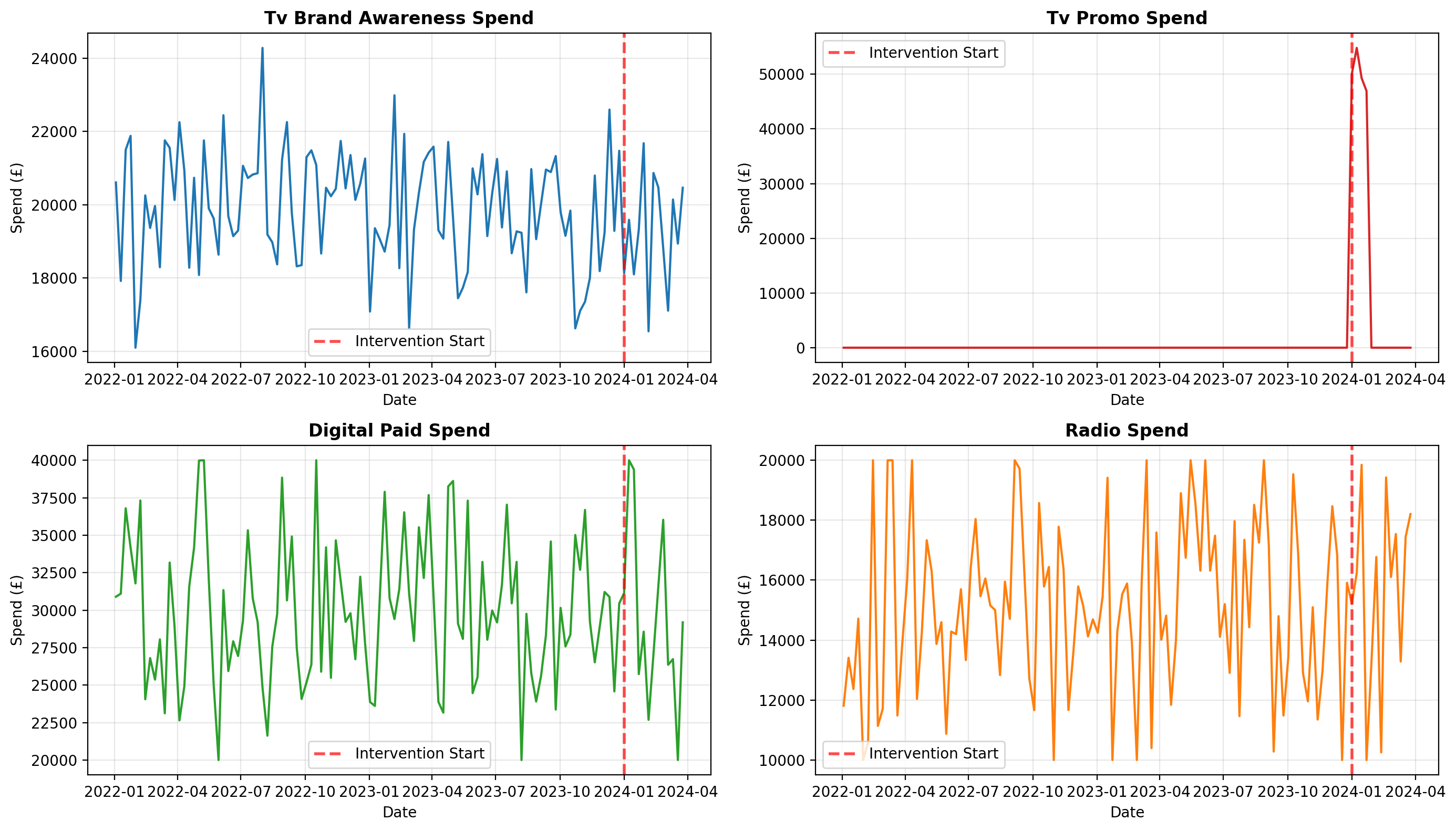
2. Generate Media Spend Data#

We’ll create spend data for four media channels, each with realistic patterns.

# Initialize spend arrays
spend_data = {}

# 1. TV Brand Awareness: constant low-level spend throughout
# Baseline TV spend around £20,000/week with small random variation
spend_data["tv_brand_awareness"] = 20_000 + rng.normal(0, 2_000, n_total)
spend_data["tv_brand_awareness"] = np.clip(
    spend_data["tv_brand_awareness"], 15_000, 25_000
)

# 2. TV Promo: zero pre-intervention, high spend for 4 weeks during intervention
spend_data["tv_promo"] = np.zeros(n_total)
# High spend during first 4 weeks of intervention (weeks 104-107)
promo_weeks = 4
for i in range(promo_weeks):
    # Promo spend around £50,000/week (much higher than baseline)
    spend_data["tv_promo"][n_weeks_pre + i] = 50_000 + rng.normal(0, 3_000)

# 3. Digital Paid: steady spend with random variation
# Around £30,000/week
spend_data["digital_paid"] = 30_000 + rng.normal(0, 5_000, n_total)
spend_data["digital_paid"] = np.clip(spend_data["digital_paid"], 20_000, 40_000)

# 4. Radio: steady spend with random variation
# Around £15,000/week
spend_data["radio"] = 15_000 + rng.normal(0, 3_000, n_total)
spend_data["radio"] = np.clip(spend_data["radio"], 10_000, 20_000)

# Create dataframe
df_spend = pd.DataFrame(spend_data, index=date_range)
df_spend.head(10)

	tv_brand_awareness	digital_paid	radio
2022-01-03	20609.434160	30896.378175	11812.756764
2022-01-10	17920.031788	31099.983420	13411.681718
2022-01-17	21500.902392	36795.937876	12369.417665
2022-01-24	21881.129433	34175.556230	14717.212337
2022-01-31	16097.929623	31784.355296	10000.000000
2022-02-07	17395.640986	37316.514456	10598.864264
2022-02-14	20255.680806	24056.184728	20000.000000
2022-02-21	19367.514815	26801.242336	11137.732256
2022-02-28	19966.397685	25367.120293	11709.643265
2022-03-07	18293.912145	28050.950984	20000.000000

Let’s visualize the media spend over time, highlighting the TV promo spike:

fig, axes = plt.subplots(2, 2, figsize=(14, 8))
axes = axes.flatten()

channels = ["tv_brand_awareness", "tv_promo", "digital_paid", "radio"]
colors = ["#1f77b4", "#d62728", "#2ca02c", "#ff7f0e"]

for ax, channel, color in zip(axes, channels, colors):
    ax.plot(df_spend.index, df_spend[channel], color=color, linewidth=1.5)
    ax.axvline(
        intervention_start,
        color="red",
        linestyle="--",
        linewidth=2,
        alpha=0.7,
        label="Intervention Start",
    )
    ax.set_title(
        f"{channel.replace('_', ' ').title()} Spend", fontsize=12, fontweight="bold"
    )
    ax.set_xlabel("Date")
    ax.set_ylabel("Spend (£)")
    ax.legend()
    ax.grid(alpha=0.3)

plt.tight_layout()

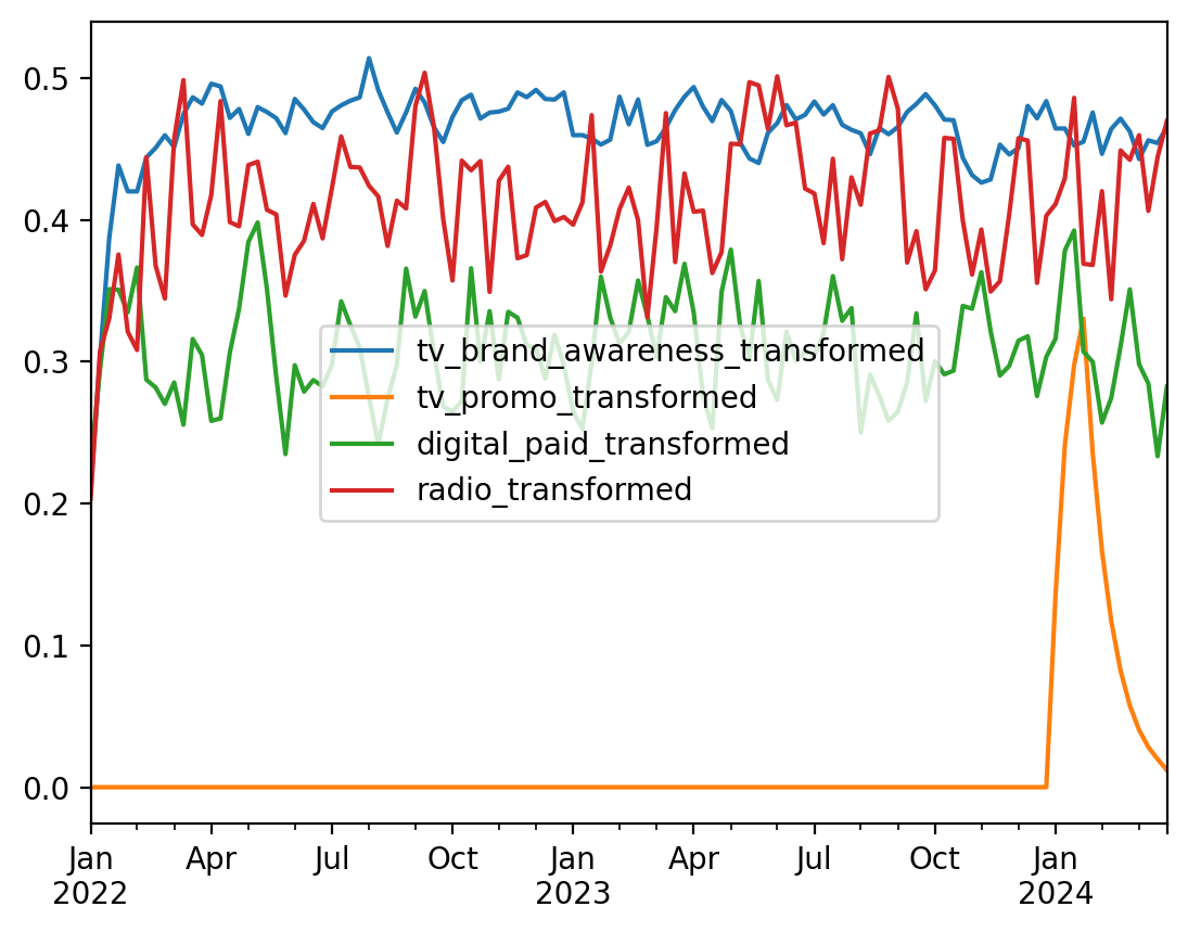
../_images/736d4b19566c2d0110c2fed7a4ca6d94f5f631f68e5be707628274407358c846.png

3. Apply Marketing Transformations#

In real-world marketing, media effects are not instantaneous or linear:

Adstock Effect: Media exposure has a carryover effect. When someone sees a TV ad, the impact on their purchase behavior extends beyond that moment and decays over time.
Saturation Effect: There are diminishing returns to advertising spend. Doubling the spend doesn’t double the impact.

We’ll use transformations from the pymc-marketing package to model these effects realistically.

# Define transformation parameters for each channel
# Different channels have different adstock (carryover) and saturation characteristics

# Adstock parameters (alpha): higher = longer carryover effect
# Saturation parameters (lam): controls the inflection point of the saturation curve

channel_params = {
    "tv_brand_awareness": {
        "alpha": 0.6,  # Moderate carryover
        "lam": 0.5,
    },
    "tv_promo": {
        "alpha": 0.7,  # Strong carryover (high impact ads are remembered longer)
        "lam": 0.3,
    },
    "digital_paid": {
        "alpha": 0.3,  # Short carryover (digital is more immediate)
        "lam": 0.6,
    },
    "radio": {
        "alpha": 0.4,  # Moderate carryover
        "lam": 0.7,
    },
}

# Apply transformations to each channel
df_transformed = pd.DataFrame(index=date_range)

for channel in channels:
    # Get channel spend
    spend = df_spend[channel].to_numpy()

    # Scale the spend using max absolute value (brings values to 0-1 range)
    # This is important because saturation functions work best with scaled inputs
    spend_max = spend.max()
    spend_scaled = spend / spend_max if spend_max > 0 else spend

    # Apply Geometric Adstock transformation
    spend_adstocked = geometric_adstock(
        x=spend_scaled, alpha=channel_params[channel]["alpha"]
    ).eval()

    # Apply Logistic Saturation transformation
    spend_transformed = logistic_saturation(
        x=spend_adstocked, lam=channel_params[channel]["lam"]
    ).eval()

    df_transformed[f"{channel}_transformed"] = spend_transformed

Transformed media features created:
Value ranges: min=0.0000, max=0.5141

	tv_brand_awareness_transformed	digital_paid_transformed	radio_transformed
2022-01-03	0.209049	0.227663	0.203828
2022-01-10	0.302070	0.293843	0.307148
2022-01-17	0.387141	0.351189	0.330529
2022-01-24	0.438465	0.350801	0.375594
2022-01-31	0.420194	0.334858	0.321185

df_transformed.plot();

<Axes: >

../_images/c7836d01fa847bf76d022086d05af3f3c994757ac0d68d5f137a1c98bcb3de92.png

4. Construct the Target Variable (Sales)#

Now we’ll build our sales data by combining all components. The sales are driven by baseline factors (trend, seasonality) plus the transformed media contributions.

# Create time index for trend
t = np.arange(n_total)

# 1. Baseline intercept (average sales with no marketing)
intercept = 5000

# 2. Linear trend (business growth over time)
trend = 10 * t  # Growing by ~10 units per week

# 3. Annual seasonality (using month of year and week of month)
# Extract month from date_range
months = date_range.month
# Create monthly seasonal component using sine waves
monthly_seasonality = 500 * np.sin(2 * np.pi * months / 12) + 300 * np.cos(
    2 * np.pi * months / 12
)

# Extract week of month (1-5, since no month has more than 31 days)
week_of_month = ((date_range.day - 1) // 7 + 1).values
# Create week of month effect (smaller amplitude than monthly)
# Different weeks of the month have different sales patterns
week_of_month_effect = np.array(
    [{1: 100, 2: 50, 3: -20, 4: -50, 5: -80}.get(w, 0) for w in week_of_month]
)

# Combined seasonality
seasonality = monthly_seasonality + week_of_month_effect

# 4. Media contributions with coefficients
# These coefficients represent the "true" effect of each channel on sales
media_coefficients = {
    "tv_brand_awareness_transformed": 0.8,
    "tv_promo_transformed": 20.5,  # TV promo has a stronger effect
    "digital_paid_transformed": 1.2,
    "radio_transformed": 0.6,
}

media_contribution = np.zeros(n_total)
for channel, coef in media_coefficients.items():
    media_contribution += coef * df_transformed[channel].values

# 5. Random noise
noise_sigma = 200
noise = rng.normal(0, noise_sigma, n_total)

# Combine all components to create sales
sales = intercept + trend + seasonality + media_contribution + noise

# Create the final dataframe
df = pd.DataFrame(
    {
        "date": date_range,
        "sales": sales,
        "t": t,
        "month": months,
        "week_of_month": week_of_month,
    }
)

# Add a column to indicate intervention period
df["post_intervention"] = (df["date"] >= intervention_start).astype(int)

# Set date as index
df = df.set_index("date")

print("Sales statistics:")
print(f"Mean: {df['sales'].mean():.2f}")
print(f"Std: {df['sales'].std():.2f}")
print(f"Min: {df['sales'].min():.2f}")
print(f"Max: {df['sales'].max():.2f}")

df.head()

Sales statistics:
Mean: 5639.30
Std: 584.24
Min: 4395.50
Max: 7042.70

First few rows:

	sales	t	month	week_of_month	post_intervention
date
2022-01-03	5656.945956	0	1	1	0
2022-01-10	5617.466355	1	1	2	0
2022-01-17	5564.805726	2	1	3	0
2022-01-24	5318.135657	3	1	4	0
2022-01-31	5441.232581	4	1	5	0

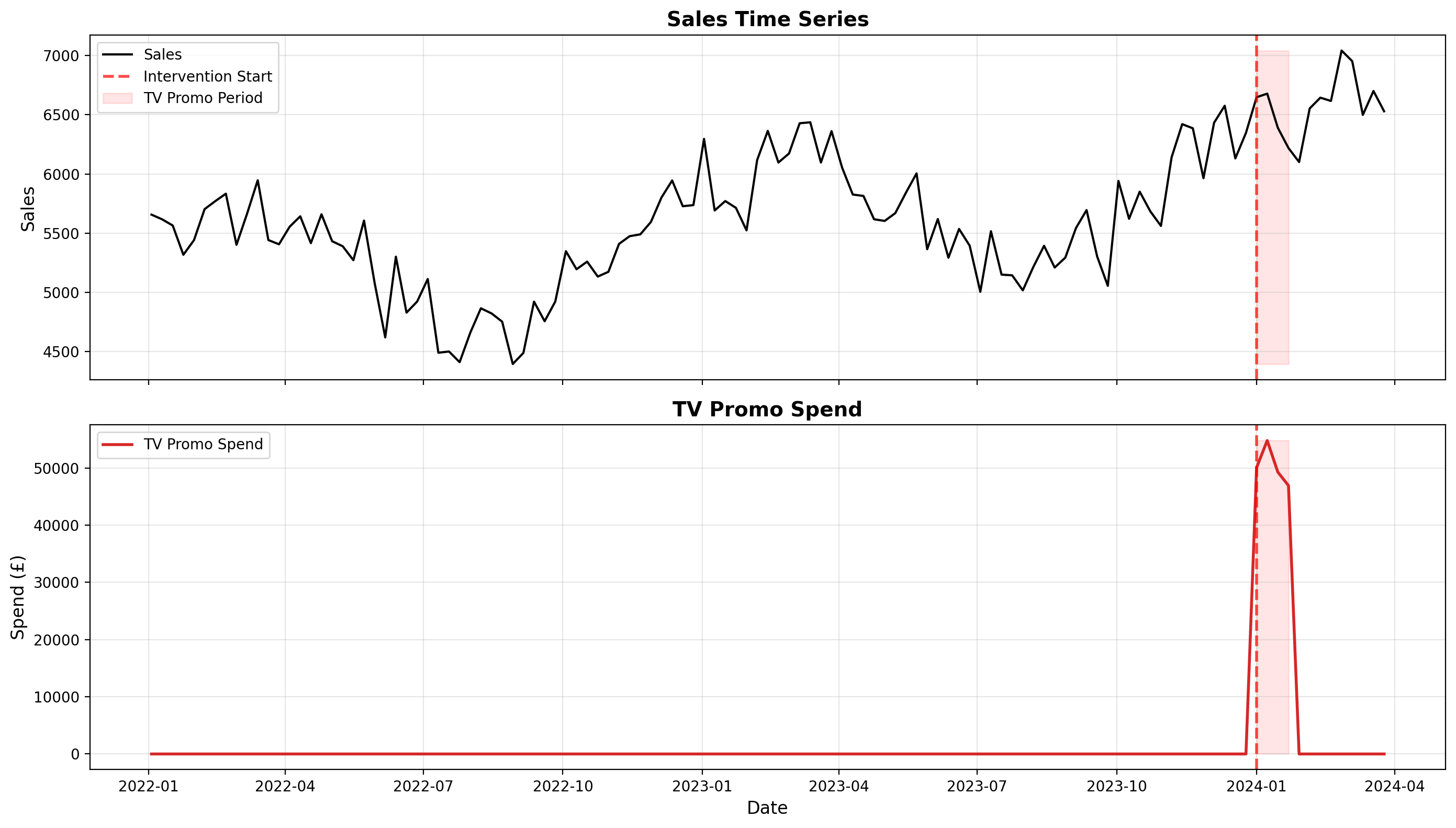
5. Visualize the Data#

Let’s visualize the sales time series and see if we can spot the impact of the TV promo campaign.

../_images/31678fbfcf0a6184cdeded2c58820149acbfc7bf02ec8ac1048a267fe967e651.png

Part II: Interrupted Time Series Analysis#

Now that we have our simulated data, we can use CausalPy’s Interrupted Time Series method to estimate the causal impact of the TV promo campaign.

The key insight of ITS is:

We fit a model to the pre-intervention period (before the TV promo)
We use this model to predict what would have happened in the post-intervention period (the counterfactual)
We compare the actual observed sales to the counterfactual to estimate the causal impact

Note that we do not include the TV promo spend in our ITS model. We’re trying to estimate the total impact of the intervention, regardless of which specific factors drove it. The ITS model will capture the baseline trends and seasonality to create an accurate counterfactual.

Run the ITS Analysis#

We’ll fit a model that includes a time trend, monthly seasonality, and week-of-month effects to capture the baseline sales pattern.

The formula "sales ~ 1 + t + C(month) + C(week_of_month)" specifies a linear regression model with the following components:

1: Intercept term (baseline level of sales)
t: Linear time trend to capture long-term growth or decline
C(month): Categorical variable for month of year (1-12)
- Creates 11 dummy variables (with one month as reference)
- Captures annual seasonality patterns (e.g., higher sales in summer, lower in winter)
C(week_of_month): Categorical variable for week within month (1-5)
- Creates 4 dummy variables (with week 1 as reference)
- Captures within-month patterns (e.g., beginning vs end of month effects)

This modeling approach is deliberately simple and interpretable. We’re using categorical variables rather than smooth functions (like splines or Fourier terms) because:

Flexibility: Each month and week can have its own level without constraining the pattern
Robustness: Less prone to overfitting than complex non-linear models
Interpretability: Easy to understand which time periods have higher/lower baseline sales

The key assumption is that these baseline patterns (trend + seasonality) would have continued unchanged in the post-intervention period if the TV promo hadn’t occurred. Any deviation from this pattern is attributed to the campaign.

Note

The random_seed keyword argument for the PyMC sampler is not necessary. We use it here so that the results are reproducible.

result = cp.InterruptedTimeSeries(
    df,
    treatment_time=intervention_start,
    formula="sales ~ 1 + t + C(month) + C(week_of_month)",
    model=cp.pymc_models.LinearRegression(sample_kwargs={"random_seed": seed}),
)

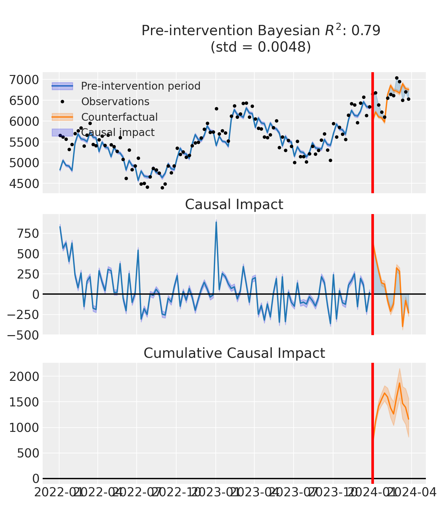
Visualize the Results#

fig, ax = result.plot()

../_images/3eaa16c0eb27772d00f5497ee7f49cab46769fd806f53b2316c3555abeac8c68.png

Let’s also look at the model summary:

result.summary()

==================================Pre-Post Fit==================================
Formula: sales ~ 1 + t + C(month) + C(week_of_month)
Model coefficients:
    Intercept              4828, 94% HDI [4795, 4859]
    C(month)[T.2]          583, 94% HDI [547, 618]
    C(month)[T.3]          579, 94% HDI [541, 615]
    C(month)[T.4]          293, 94% HDI [256, 332]
    C(month)[T.5]          125, 94% HDI [91, 157]
    C(month)[T.6]          -250, 94% HDI [-288, -213]
    C(month)[T.7]          -547, 94% HDI [-583, -511]
    C(month)[T.8]          -508, 94% HDI [-543, -471]
    C(month)[T.9]          -473, 94% HDI [-511, -434]
    C(month)[T.10]         -145, 94% HDI [-180, -110]
    C(month)[T.11]         128, 94% HDI [93, 166]
    C(month)[T.12]         291, 94% HDI [255, 328]
    C(week_of_month)[T.2]  214, 94% HDI [188, 240]
    C(week_of_month)[T.3]  85, 94% HDI [59, 110]
    C(week_of_month)[T.4]  55, 94% HDI [30, 81]
    C(week_of_month)[T.5]  -60, 94% HDI [-96, -23]
    t                      11, 94% HDI [11, 12]
    y_hat_sigma            49, 94% HDI [48, 50]

Part III: Calculating Lift Test Results#

This section extracts the lift test results from our ITS analysis. The result object contains the post-intervention impact estimates in the post_impact attribute, which stores the full posterior distribution of the causal effect at each time point.

These results can be used in two ways:

Immediate evaluation: Assess this specific campaign’s performance
MMM calibration: Feed these experimental results into your Media Mix Model to improve attribution accuracy

1. Absolute Lift (Primary Output for MMM Calibration)#

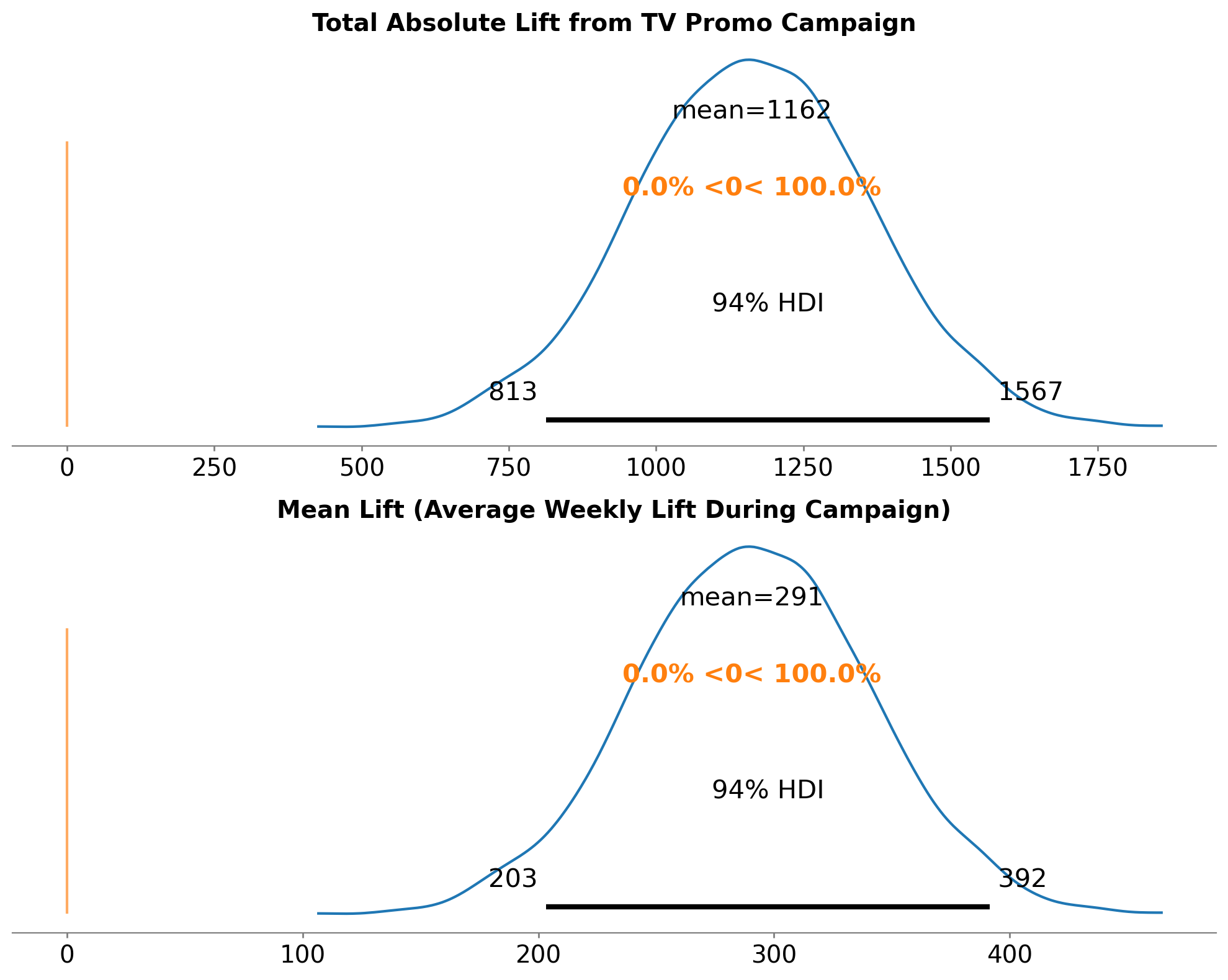
The absolute lift is the total incremental units (sales, conversions, etc.) attributable to the intervention. This is calculated by summing the post-intervention impact across all post-intervention time points.

For MMM Calibration: The mean and standard deviation of this lift distribution are the key inputs needed. These tell your MMM:

How much lift was actually observed from the campaign (mean)
How uncertain we are about that estimate (standard deviation)

The MMM uses this information to calibrate its saturation curves, ensuring the model’s predictions align with real-world experimental evidence.

../_images/01db2e241ce76c2c5a6ed9d3180a0e82b5ba28615d48a321cf9b38df0514748a.png

Absolute Lift Summary:
               mean       sd   hdi_3%   hdi_97%
x[unit_0]  1162.383  199.045  813.024  1566.653

Most credible estimate: 1162.38 incremental sales
94% Credible Interval: [813.02, 1566.65]

Key Outputs for MMM Calibration

From the absolute lift calculation above, extract these values for MMM calibration:

Mean Lift (delta_y): The mean value from the summary table (e.g., 1162.38 incremental sales)
Standard Deviation (sigma): The sd value from the summary table (e.g., 199.05)
Spend Increment (delta_x): The weekly spend during the test - can be expressed as:
- Absolute: £50,000/week (actual spend during promo)
- Normalized: Depends on your MMM’s scaling (e.g., if max weekly spend in your data is £150k, then 50k/150k = 0.33)
Baseline Spend (x): The spend level before the increment - in this case, £0 for tv_promo (or 0.0 normalized)

Important: The choice between absolute and normalized values depends on how your MMM preprocesses media spend data. If your MMM normalizes spend by dividing by the maximum, use normalized values. If it uses raw spend, use absolute values.

Example formatting for PyMC-Marketing (which typically expects normalized values):

# Calculate normalized values based on your MMM's scaling
max_weekly_spend = 150_000  # Maximum weekly spend in your MMM training data
promo_spend_weekly = 50_000  # Weekly spend during this test

lift_test_df = pd.DataFrame({
    "channel": ["tv_promo"],
    "x": [0.0],  # Baseline spend for tv_promo (normalized) - it's zero before test
    "delta_x": [promo_spend_weekly / max_weekly_spend],  # Spend increment (normalized) = 0.33
    "delta_y": [1162.38],  # Mean lift from ITS result
    "sigma": [199.05]  # Std of lift from ITS result
})

Alternative: Some MMM implementations may expect the actual spend level (x + delta_x) rather than the increment. Check your MMM’s documentation for the expected format.

See the PyMC-Marketing lift test calibration guide for complete integration details.

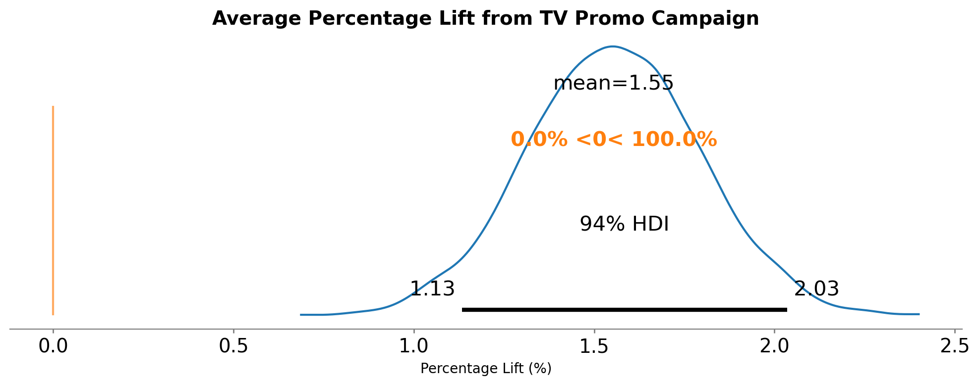
2. Percentage Lift#

The percentage lift tells us by what percentage the campaign increased sales compared to what would have happened without it. This is calculated as:

\[\text{Percentage Lift} = \frac{\text{Observed Sales} - \text{Counterfactual Sales}}{\text{Counterfactual Sales}} \times 100\]

../_images/2d5a42f4a39f4fa0f6f68abffb90884eb648151ae47fae9b601049cf710438d3.png

Percentage Lift Summary:
            mean     sd  hdi_3%  hdi_97%
x[unit_0]  1.554  0.238   1.134    2.035

Most credible estimate: 1.55% lift
94% Credible Interval: [1.13%, 2.04%]

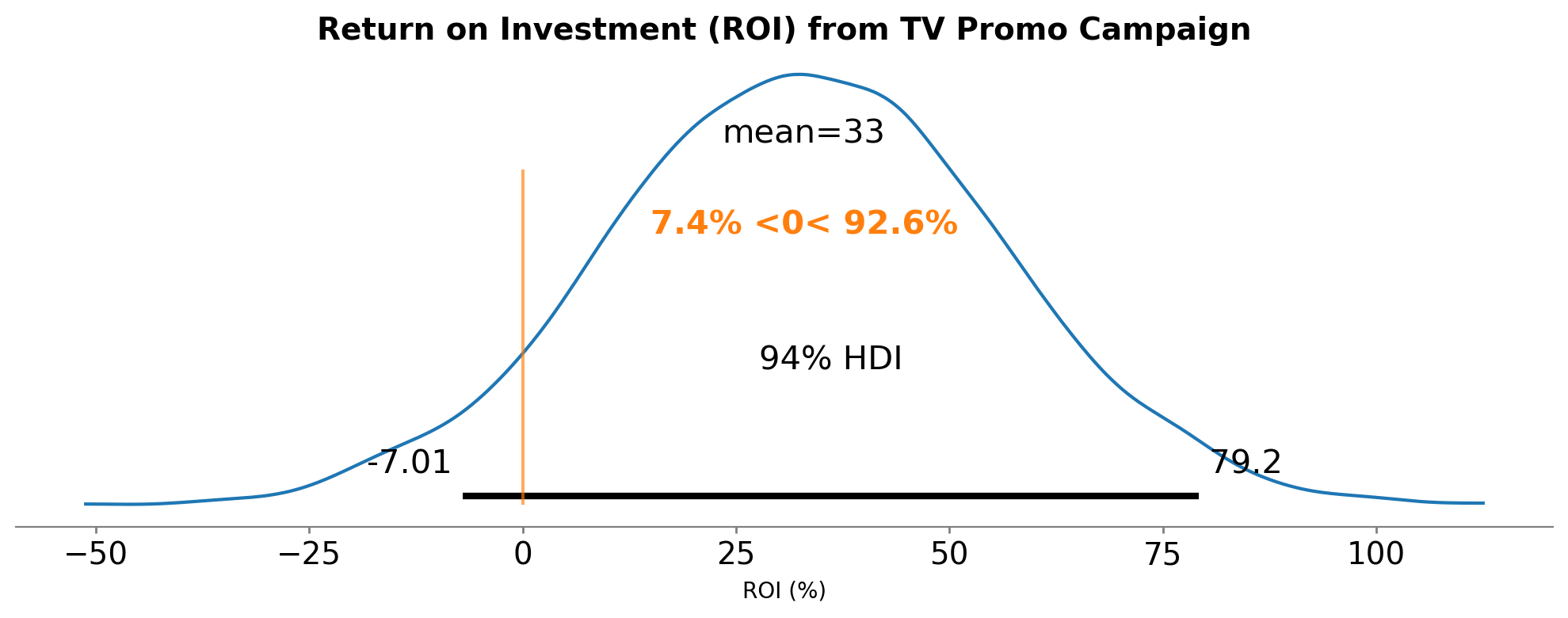
3. Return on Investment (ROI)#

Finally, let’s calculate the ROI of the TV promo campaign. We need to:

Calculate the total spend on the TV promo campaign
Calculate the incremental revenue (absolute lift × revenue per unit)
Compute ROI as: \(\text{ROI} = \frac{\text{Incremental Revenue} - \text{Campaign Spend}}{\text{Campaign Spend}} \times 100\)

For this example, let’s assume each unit of sales generates £230 in revenue.

Total TV Promo Spend: £201,082.33

../_images/74944476387b261ff6e394ea3fd22c0ff50774eb919d904ac0ea18f98f0d7fd5.png

ROI Summary:
             mean      sd  hdi_3%  hdi_97%
x[unit_0]  32.955  22.767  -7.005   79.195

Most credible estimate: 32.95% ROI
94% Credible Interval: [-7.00%, 79.19%]

--- Financial Summary ---
Campaign Spend: £201,082.33
Incremental Revenue (mean): £267,348.02
Net Profit (mean): £66,265.69

Summary and Interpretation#

What Did We Learn from This Lift Test?#

Using Interrupted Time Series analysis, we successfully conducted a lift test and generated experimental evidence about the TV promo campaign’s causal impact. Here’s what we extracted:

Primary Lift Test Output (for MMM Calibration):

Absolute Lift: Mean = ~1,162 incremental sales, SD = ~199 sales
These values (mean and SD) can be directly fed into MMM calibration procedures

Additional Business Insights:

Percentage Lift: Approximately 1.4% average lift over the post-intervention period
ROI: Approximately 33% return on investment, with wide credible intervals reflecting uncertainty

This experimental evidence provides ground truth data that your MMM can use to calibrate its response curves, ensuring the model’s predictions align with real-world results.

The Power of Adstock Effects#

Notice in the middle panel of the ITS plot that the impact doesn’t immediately drop to zero after the 4-week campaign ends. This is because:

The adstock effect means that TV advertising has carryover—people remember the ads for weeks after seeing them
Our ITS model captures this delayed impact by measuring the difference between observed and counterfactual sales throughout the entire post-intervention period

This is exactly why we included 3 months of post-intervention data rather than just the 4 weeks of active spending.

Business Implications#

This analysis provides actionable insights for marketing decision-makers:

Campaign Effectiveness: The credible intervals tell us how confident we can be in the lift estimates. Narrow intervals mean more certainty; wide intervals suggest more uncertainty and possibly a need for more data or a larger effect size.
Budget Optimization: The ROI metric directly informs whether similar campaigns should be repeated, scaled up, or reconsidered. A positive ROI (with credible intervals excluding zero) provides strong evidence for continuing the strategy.
Separating Baseline from Promo: By keeping baseline TV brand awareness separate from the promo campaign, we can accurately attribute the incremental lift to the specific intervention rather than confounding it with ongoing activities.
Future Experiments: If the credible intervals are wide, consider running similar campaigns in different time periods to gather more evidence, or consider increasing the campaign intensity to create a larger, more detectable signal.

Assumptions and Limitations#

As with any causal inference method, ITS relies on certain assumptions:

Key Assumptions:

No Other Interventions: We assume no other major changes occurred at the same time as the TV promo campaign. If a competitor launched a major product or there was an economic shock, this could bias our estimates.
Correct Model Specification: Our ITS model includes trend and seasonality. If the pre-intervention data has other patterns (e.g., sudden regime changes, non-linear trends), we’d need to adjust the model accordingly.
Stable Relationships: We assume the relationship between time, seasonality, and sales would have continued in the same pattern without the intervention.

Limitations:

Single Time Series: Unlike geographic experiments (e.g., GeoLift), we only have one time series, so we can’t control for contemporaneous shocks that affect all units equally.
No Synthetic Control: If we had similar control markets, we could use Synthetic Control methods for additional robustness.
Effect Heterogeneity: ITS gives us an average treatment effect. If the effect varied over time in complex ways, we might need more sophisticated time-varying effect models.

Despite these limitations, ITS remains one of the best tools available when geographic controls are unavailable.

Using Lift Test Results for MMM Calibration#

The primary purpose of running lift tests is to generate experimental evidence that can improve your Media Mix Models. Here’s how to use these results:

1. Feed Results into MMM Calibration#

The mean and standard deviation of the absolute lift (extracted above) can be directly integrated into MMM frameworks like PyMC-Marketing using the add_lift_test_measurements() method. This:

Constrains the MMM’s saturation curves to match observed experimental data
Improves parameter identifiability, especially for correlated channels
Provides more accurate attribution and ROI estimates

See the PyMC-Marketing lift test calibration documentation for implementation details.

2. Run Multiple Lift Tests#

To get the most value from lift testing:

Test different channels to calibrate each saturation curve
Test at different spend levels to better define the curve shape
Run tests in different time periods to capture seasonal variations
Accumulate results over time to build a robust calibration dataset

3. Additional Extensions#

Incorporating Other Data: Include additional predictors (weather, competitors, events) in the ITS model to improve counterfactual accuracy
Time-Varying Effects: Examine result.post_impact at individual time points to understand how effects decay over time
Hierarchical Models: If you have multiple products or sub-markets, pool information across units while estimating unit-specific lift

Conclusion#

This notebook demonstrated how to conduct lift tests using Interrupted Time Series analysis when traditional control groups are unavailable. We showed how ITS can measure the causal impact of a national TV campaign, extracting the key statistical outputs (mean lift and standard deviation) that are essential for Media Mix Model calibration. Beyond these primary outputs, we also calculated percentage lift and ROI to provide immediate business insights for decision-makers.

The importance of lift testing extends beyond measuring individual campaigns. Lift tests provide experimental evidence that validates whether your marketing actually works, separating signal from noise in your attribution models. When these experimental results are fed into MMM calibration procedures, they constrain the model’s saturation curves to match real-world observations, dramatically improving parameter identifiability—especially for correlated channels where the model might otherwise struggle to distinguish their individual effects. This leads to more accurate attribution estimates and better-informed budget allocation decisions.

The Complete Lift Testing Workflow

For a complete marketing analytics workflow, lift testing fits into a three-step process:

Run lift tests (this notebook) → Generate experimental evidence using ITS to measure the true causal impact of campaigns
Calibrate your MMM → Feed lift test results into your Media Mix Model using methods like PyMC-Marketing’s add_lift_test_measurements() to constrain model parameters
Optimize budget → Use the calibrated MMM to allocate marketing spend across channels with confidence that the model reflects real-world effectiveness

This approach bridges the gap between experimental causal inference and predictive modeling, combining the rigor of randomized experiments with the practical needs of ongoing attribution and optimization.

The method shown here is particularly valuable for national-level campaigns where geographic controls don’t exist, but it can be extended in several ways. Multiple lift tests can be accumulated over time—testing different channels, different spend levels, and different time periods—to build a robust calibration dataset. The ITS model itself can be enhanced by incorporating additional predictors like weather, competitor activity, or special events to improve the counterfactual’s accuracy. For organizations with multiple products or sub-markets, hierarchical Bayesian models can pool information across units while still estimating unit-specific lift.

Ultimately, this approach represents a practical solution to one of marketing’s most challenging problems: measuring incrementality when traditional experimental designs aren’t feasible. By combining the strengths of time series analysis with Bayesian uncertainty quantification, we can generate the experimental evidence needed to build better attribution models and make more confident investment decisions.